 +
+
chDB v4: The Fastest SQL Engine
on Pandas DataFrame
Zero-Copy Architecture · DataStore API · Benchmarks
Auxten Wang · Technical Director @ ClickHouse
ClickHouse Release 26.3 Webinar · 15 min
What is chDB?
No server needed
pip install chdbZero config
JOINs, CTEs, Window
CSV, Parquet, S3...
import chdb
import pandas as pd

df = pd.DataFrame({'user_id': range(1_000_000),
                    'category': ['A', 'B', 'C'] * 333334})

result = chdb.query("""
    SELECT category, COUNT(*) as cnt
    FROM Python(df)
    GROUP BY category
""", "DataFrame")
Same ClickHouse engine you already know — compiled as a shared library, embedded in your Python process. No infrastructure.
The Problem: Pandas at Scale
"I have a DataFrame. I want to run SQL on it. Give me back a DataFrame. Fast."
- Single-threaded. One core out of 16 doing the work
- Eager execution. Every step materializes the full result in memory
- Memory hungry. A 50M-row JOIN peaks at 10.5 GB in Pandas
On an 8 GB laptop, that JOIN will OOM and kill your process.
What if you could keep writing Pandas code, but run it up to 247x faster with 23x less memory?
The Journey to Zero-Copy
DataFrame → Parquet → CH → Parquet → DataFrame
Direct memory read from DataFrame
Output still via Parquet
DataFrame ↔ ClickHouse ↔ DataFrame
No serialization anywhere
Three generations of engineering to eliminate every serialization bottleneck
Is chDB Fast?
chDB is ClickHouse — same codebase, same vectorized engine, same SIMD pipelines.
So how do we make it the fastest SQL engine on Pandas DataFrame?
NumPy arrays in memory
serialization, GIL, encoding
already blazing fast
The secret: Don't let Python slow down ClickHouse.
- Zero serialization — read/write DataFrame memory directly
- Minimize GIL — batch all Python calls, then release
- Bypass CPython — rewrite hot paths (string encoding) in C++
The next 3 slides show exactly how we did each of these.
How Zero-Copy Works
Input: DataFrame → ClickHouse
- Extract raw pointers from NumPy arrays
- Map NumPy dtypes to ClickHouse types
- ClickHouse reads memory directly — no copy
Output: ClickHouse → DataFrame
- Map ClickHouse column types to NumPy dtypes
- Share underlying memory buffers directly
- SIMD-optimized batch conversion for results
For numeric-heavy workloads, the boundary crossing cost is effectively constant, regardless of data size
Breakthrough 1: GIL Two-Phase Design
The problem: ClickHouse wants all 16 cores. Python's GIL says "one thread at a time."
If we call CPython API per data access → multi-threaded engine degrades to single-threaded.
prepareColumnCache()Hold GIL → extract
buf, stride, dtype for every columnOne batch of Python calls, then done
PythonSource streamsEach stream reads its row slice via
col.buf + offsetNo GIL, no Python API — pure pointer arithmetic
// Phase 1: prepareColumnCache() — GIL held
{
    py::gil_scoped_acquire acquire;
    for (auto & col : column_cache) {
        // Pandas: df[col].to_numpy() → array
        py::array arr = column.attr("to_numpy")();
        col.buf    = arr.data();   // raw pointer
        col.stride = arr.strides(0);
        col.row_count = arr.size();
    }
}  // GIL released — shared across all streams

// Phase 2: N parallel PythonSource streams
// each reads a row slice via raw pointer math
void insert_from_ptr(const void* ptr,
    MutableColumnPtr& col, size_t offset,
    size_t count, size_t stride) {
    // Direct memcpy — no GIL, no Python API
    const char* start = (char*)ptr
                        + offset * sizeof(T);
    col->appendRawData(start, count);
}
One GIL acquisition to cache all pointers → N parallel streams read raw memory
Breakthrough 2: C++ String Encoding
The problem: Python str stores as Latin-1, UCS-2, or UCS-4 internally (PEP 393). ClickHouse expects UTF-8.
Calling PyUnicode_AsUTF8 requires holding the GIL. Millions of strings → entire conversion becomes serial.
GIL per string → serial
8.6s
Direct memory, parallel
0.56s
15x faster on Q23 (SELECT * WHERE URL LIKE '%google%' ORDER BY EventTime)
// Step 1: Get raw pointer + kind without
// Python C API (via pybind11 non_limited_api)
getPyUnicodeUtf8(obj, data, length,
                 kind, codepoint_cnt,
                 direct_insert);

// Step 2: Convert in C++ — no GIL needed
static size_t ConvertPyUnicodeToUtf8(
    const void* input, int kind,
    size_t codepoint_cnt,
    Offsets& offsets, Chars& chars) {
  switch (kind) {
  case 1: // Latin-1 (1 byte/char)
    for (size_t i = 0; i < codepoint_cnt; ++i)
      offset += utf8proc_encode_char(
        ((uint8_t*)input)[i], &chars[offset]);
    break;
  case 2: // UCS-2 (2 bytes/char)
    for (size_t i = 0; i < codepoint_cnt; ++i)
      offset += utf8proc_encode_char(
        ((uint16_t*)input)[i], &chars[offset]);
    break;
  case 4: // UCS-4 (4 bytes/char)
    /* same pattern with uint32_t */
  }
}
Breakthrough 3: Native JSON on DataFrame
The problem: Real DataFrames often have object columns filled with nested dicts. Traditional approach: flatten to columns first, lose structure.
chDB's approach:
- Sample
objectcolumn to detect dict structure - Auto-map to ClickHouse's native JSON type
- Query nested fields with dot notation — no flattening
- Full access to ClickHouse JSON functions
import pandas as pd, chdb

data = pd.DataFrame({
    'event': [
        {'type': 'click',
         'meta': {'x': 100, 'y': 200}},
        {'type': 'scroll',
         'meta': {'x': 150, 'y': 300}},
        {'type': 'click',
         'meta': {'x': 200, 'y': 400}}
    ]
})

# Dot notation on nested JSON!
result = chdb.query("""
    SELECT
        event.type,
        event.meta.x AS x_coord,
        event.meta.y AS y_coord
    FROM Python(data)
    WHERE event.type = 'click'
""", "DataFrame")

#   event.type  x_coord  y_coord
# 0      click      100      200
# 1      click      200      400
Perfect for log analytics, event data, API responses — no pre-processing, no schema definition
Your Pandas Code
One Line Change
Under the Hood
Inside the Engine
SELECT city,
       AVG(salary) AS mean,
       SUM(salary) AS sum,
       COUNT(salary) AS count
FROM file('employee_data.csv',
          'CSVWithNames')
WHERE age > 25
  AND salary > 50000
GROUP BY city
ORDER BY mean DESC
LIMIT 10
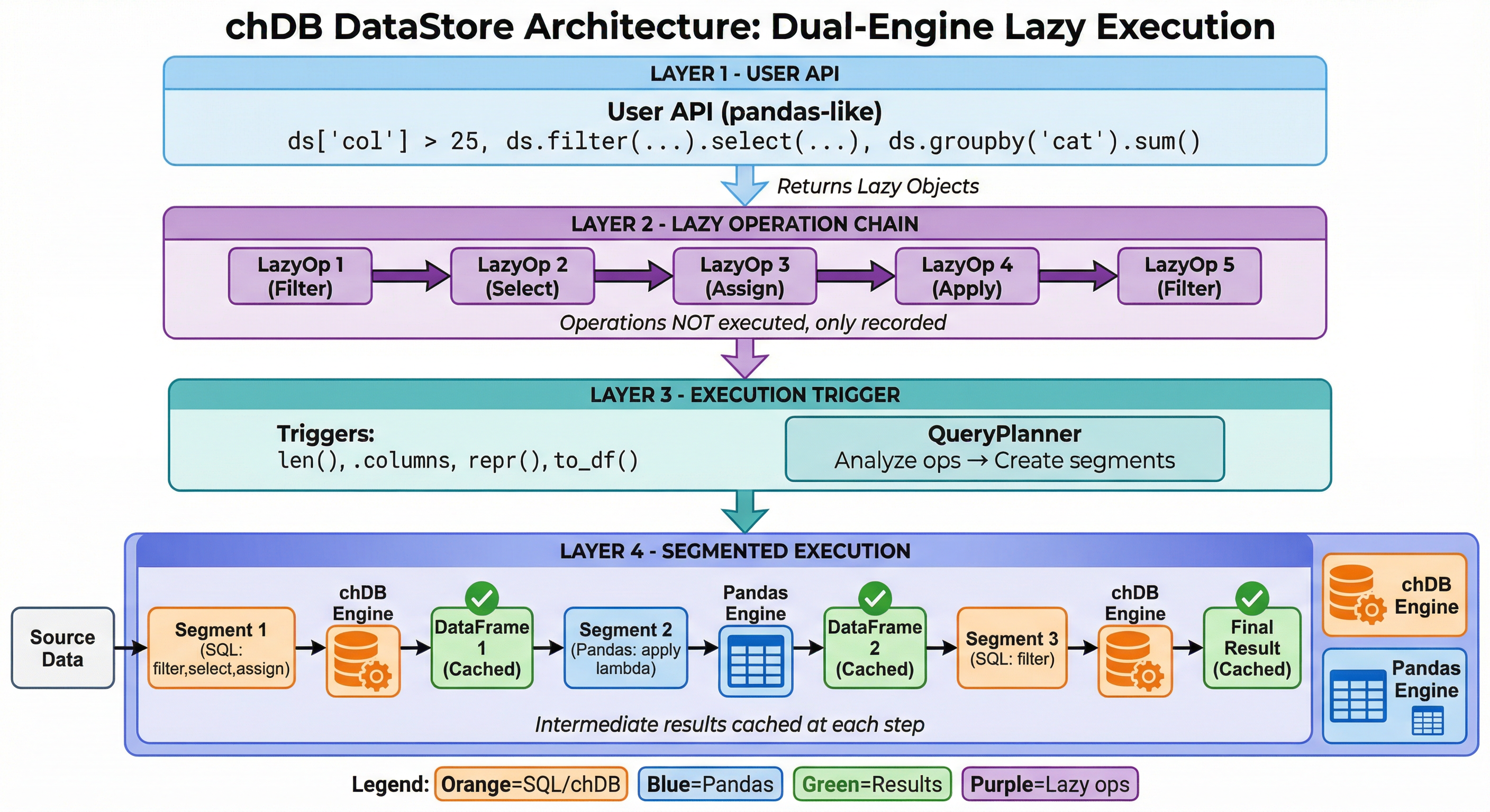
DataStore: Four-Layer Architecture
Layer 1 — Pandas API
ds['col'] > 25, ds.groupby(), ds.merge()
Every call returns a lazy object
Layer 2 — LazyOp Chain
Records operations without touching data
filter, select, assign, apply, groupby...
Layer 3 — Query Planner
Triggered by print(), len(), .columns
Splits pipeline into segments, routes to engine
Layer 4 — Execution
chDB segments ↔ Pandas segments
DataFrames flow via memoryview
Lazy Execution & explain()
from chdb import DataStore

ds = DataStore.from_file("users.parquet")
ds = ds[ds["age"] > 30]
ds = ds.sort_values("salary",
                     ascending=False)
ds = ds.head(100)

# Nothing has executed yet!
print(ds.explain())
Execution Plan
════════════════════════════════
 [1] File: users.parquet

Operations:
────────────────────────────────
 [2] [chDB] WHERE: age > 30
 [3] [chDB] ORDER BY: salary DESC
 [4] [chDB] LIMIT: 100
What happens at execution
- Filter pushdown — WHERE before reading all data
- Column pruning — only read columns you use
- Limit propagation — stop after 100 rows
- Single pass over the file, vectorized SIMD
Smart Caching
- Each
print()triggers execution & caches results - Next operation reuses the cache
- Auto-invalidated when pipeline changes
- No manual
.cache()needed
Segment Execution: Best of Both Worlds
ds = DataStore.from_file("data.parquet")
ds = ds[ds["age"] > 25]                    # → chDB segment
ds["name_upper"] = ds["name"].str.title()   # → Pandas segment (str.title)
ds = ds.sort_values("age")                  # → chDB segment
FROM file() WHERE age > 25
name.str.title()
via Python() ORDER BY age
- Auto-splits the pipeline at SQL/Pandas boundaries
- ClickHouse handles what it can; Pandas handles the rest (300+ CH functions + full Pandas ecosystem)
- Seamless handoff via Python
memoryview— for numeric data, effectively zero-copy - Tip: keep Pandas-only ops toward the end for best optimization
The query planner sees through the entire pipeline. You just write Pandas.
Unified Data Sources
DataStore inherits all of ClickHouse's data source support:
# Local files — Parquet, CSV, JSON, ORC...
ds = DataStore.from_file("events.parquet")

# Remote S3
ds = DataStore.uri("s3://bucket/path/to/data.parquet")

# Query a PostgreSQL table
ds = DataStore.from_sql("SELECT * FROM users", engine="postgresql://...")

# Mix sources in a single query — ClickHouse optimizes the execution
ds = DataStore.from_sql("""
    SELECT u.name, e.event_type, e.timestamp
    FROM file('users.parquet') u
    JOIN postgresql('host:5432', 'db', 'events', 'user', 'pass') e
    ON u.id = e.user_id
""")

ds = ds[ds["event_type"] == "purchase"].sort_values("timestamp")
print(ds)  # Lazy — executes here
80+ formats. Local, remote, in-memory, cross-database JOINs. Same Pandas-style pipeline. No ETL.
Benchmark: chDB vs Pandas — Speed & Memory (50M Rows)
| Scenario | Pandas | chDB | Speedup | Pandas Mem | chDB Mem | Mem Saved | |
|---|---|---|---|---|---|---|---|
| T01 | Read Parquet + COUNT | 2.07s | 0.28s | 7.4x | 5,310 MB | 234 MB | 22.7x |
| T02 | Filter + GroupBy + SUM | 2.88s | 0.69s | 4.1x | 7,161 MB | 1,216 MB | 5.9x |
| T03 | Multi-key GroupBy + 4 aggs | 5.31s | 1.88s | 2.8x | 7,309 MB | 4,222 MB | 1.7x |
| T04 | JOIN (50M × 10K) + agg | 6.76s | 0.87s | 7.7x | 10,473 MB | 1,824 MB | 5.7x |
| T05 | Top-10 per group (window) | 35.05s | 9.29s | 3.8x | 5,797 MB | 2,715 MB | 2.1x |
| T06 | P95 quantile by region | 4.14s | 0.68s | 6.1x | 3,699 MB | 1,472 MB | 2.5x |
| T07 | Derived cols + filter + Top-1000 | 2.93s | 1.14s | 2.6x | 7,374 MB | 2,961 MB | 2.5x |
| T08 | Count Distinct (exact) | 7.57s | 1.38s | 5.5x | 3,650 MB | 3,212 MB | 1.1x |
| T09 | In-memory DataFrame query | 2.89s | 2.17s | 1.3x | 6,841 MB | 5,550 MB | 1.2x |
| T10 | Time-series monthly agg | 4.07s | 0.68s | 6.0x | 3,216 MB | 1,679 MB | 1.9x |
/proc VmHWM
chDB wins 10/10 on speed (geomean 4.2x) and 10/10 on memory (geomean 2.9x). T04 JOIN: Pandas peaks at 10.5 GB → OOM on 8 GB laptop; chDB uses 1.8 GB → OK.
Output Zero-Copy: chDB vs DuckDB
Query ClickBench hits (1M rows) → export to Pandas DataFrame
Why chDB wins on output
- Direct type mapping — ClickHouse columns → NumPy dtypes, no intermediate format
- Memory sharing — numeric buffers shared via
memoryview, not copied - SIMD batch conversion — result chunks converted with vectorized routines
- DuckDB still serializes through its own Arrow/Pandas bridge
SELECT * FROM file('hits_0.parquet') → DataFrame
Hardware: AWS EC2 c6a.4xlarge
Method: best of 3 runs
AI Writes Pandas. chDB Runs It Fast.
- Pandas is the #1 data API in LLM training data — models generate excellent Pandas code
- DataStore executes it on ClickHouse automatically
- No need to teach your AI a new API — works with Hex AI agents, Claude, ChatGPT
The future workflow:
Pandas code
compiles to SQL
executes fast
"Hey Claude, group sales by region and show top 10."
↓ generates standard Pandas code ↓
↓ runs on ClickHouse via DataStore ↓
↓ up to 247x faster ↓
Summary: What chDB v4 Delivers
4.2x
geometric mean speedup over Pandas
across 10 real-world scenarios (50M rows)
24%
faster than DuckDB
on DataFrame export (same dataset, same hardware)
2.9 – 23x
less peak memory vs Pandas
Pandas OOM on 8 GB → chDB runs fine
0 ser/deser
complete zero-copy loop
DataFrame ↔ ClickHouse ↔ DataFrame
For ClickHouse users: chDB brings the engine you already trust into Python notebooks, Hex, Colab — same SQL dialect, same functions, same performance. No server to deploy.
Not Just Python
chDB runs as a native library in 9 languages:
Runs everywhere — no server, no infra:
Getting Started — 30 Seconds
pip install "chdb>=4.0.0"
import chdb.datastore as pd  # swap one import, done

df = pd.read_csv("your_data.csv")

result = (
    df[df['amount'] > 100]
    .groupby('category')
    .agg({'amount': 'sum', 'order_id': 'count'})
    .sort_values('amount', ascending=False)
    .head(10)
)

result.plot(kind='bar')  # Still a real DataFrame
No server. No config. No new API to learn.
The Road Ahead
-
Native Python UDF — in-process, no subprocess
Register Python functions as ClickHouse UDFs via@chdb.funcdecorator, executed inside the vectorized pipeline with full type mapping (PR #9) -
Free-threading build (no-GIL) — Python 3.14+
chDB compiled with free-threading support, enabling true multi-threaded Python UDF execution within ClickHouse's parallel pipeline (PR #12) -
PyTorch DataLoader integration
Efficient batching, shuffling, and streaming for ML training -
Hybrid execution
Seamlessly scale from laptop to ClickHouse Cloud
Thank You!